

基于物理模型和全局优化算法的叶面积指数反演
遥感生物物理参数反演是遥感观测中非常重要的一项问题,今天我们花点时间来实现这一目标。
1 核心目标
(1)掌握基于物理模型的遥感参数反演的流程并能够独立完成参数反演。
(2)了解使用全局优化算法进行生物物理参数反演问题求解的思路。
2 主要内容
(1)任选两个不同植被类型站点,反演与地面测量数据对应时间的站点周围小区域LAI,并与基于地面测量数据的LAI进行对比分析。
(2)反演站点对应像元任意一年的LAI,并与MODIS LAI对比分析。
3 前期准备
(1)数据准备
站点数据下载:选择两个不同的植被类型的站点。本次选择的是代表森林的比利时的Sonian forest站点,以及代表草地的位于尼日尔的WANKAMA站点作为案例来进行讲解。
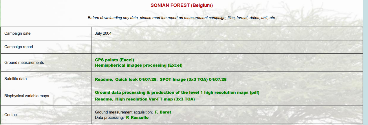
图 站点信息1

图 站点信息2
网站地址:http://w3.avignon.inra.fr/valeri/fic_htm/database/main.php.
这两个站点分别提供了UTM投影WGS-84坐标系下若干点的地面测量数据,包含有效LAI值和真实LAI值。该数据可用于后续反演LAI的精度验证。
MODIS数据下载:
首次下载,利用Global Subsets Tool工具下载小区域两个站点对应日期的地表反射率数据- MOD09A1和叶面积指数数据- MOD15A2H。两个数据的空间分辨率都是500m,由8天合成,由tif格式存储。同时下载该区域的2000-2020年MODIS的叶面积指数作为先验信息。
网站地址:TESViS Subset Order History,结果发现这个网站还是有点小问题,下载出来的影像的时间和站点观测的时间不对,这可能会影响后续的反演。
辗转多次,后面前往Google Earth Engine网站下载MODIS数据。基本流程是通过GEE平台,以站点的经纬度为中心,创建5km×5km的正方形区域,调用MODIS的反射率数据和叶面积指数产品,分别完成缩放因子操作,还原数据的数值。同时,在平台上选择站点记录的日期的每年的LAI数据,每一年在 站点观测数据对应日期附近20天窗口内的所有LAI影像先做年内平均,再对2002-2025年计算多年平均值,作为LAI反演的先验信息。
时间序列数据下载:使用Google Earth Engine网站提取Sonian forest站点所在像元的MOD09A1数据的七个波段的反射率数据和MOD15A2H的叶面积指数数据,并以表格的形式存储。
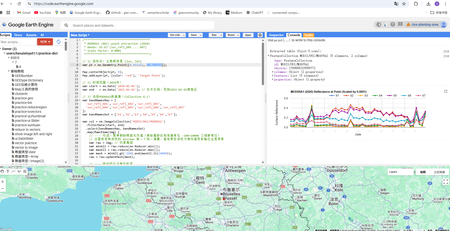
图 GEE下载站点所在像元一年七个波段的反射率数据
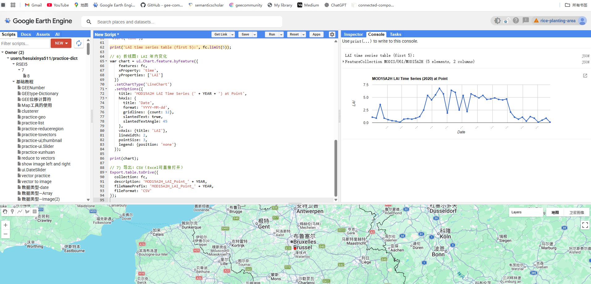
图 GEE下载站点所在像元一年的LAI数据
下载数据的代码也提供给你了,首先是下载小区域的地表反射率数据和MODIS叶面积指数产品的代码:
/*************************************************
 * ROI: 5km x 5km centered at (50.768333N, 4.411111E)
 * (1) MOD09A1 near 2004-06-21: b1-b7 scaled (0.0001), export 7 tif (one band each)
 * (2) MOD15A2H near same period: LAI scaled (0.1), export tif
 * (3) MOD15A2H prior LAI mean (2002-2025): for EACH year,
 *     mean of ALL LAI images within 6/21 ± windowDays, then multi-year mean -> export tif
 *
 * Robust strategy:
 * - Export: DO NOT use clip(); use Export.region to crop (stable)
 * - Visualization: reproject to EPSG:4326 then clip(roi) for map display
 *************************************************/

// =====================
// 0) Parameters
// =====================
var lon = 2.635278;
var lat = 13.645;

var targetDateStr = '2005-06-27'; // target date "near"
var windowDays = 20;             // "near" window in days (8-day products: 8~24)

var roiSizeKm = 5;
var halfSizeM = roiSizeKm * 1000 / 2;

var exportScale = 500;
var exportCRS = 'EPSG:4326';

// prior window mean years
var priorStartYear = 2002;
var priorEndYear   = 2025;

// =====================
// 1) ROI in EPSG:4326 rectangle (geodesic=false)
// =====================
var pt = ee.Geometry.Point([lon, lat]);

var dLat = halfSizeM / 111320;
var dLon = halfSizeM / (111320 * Math.cos(lat * Math.PI / 180));

var roi = ee.Geometry.Rectangle(
  [lon - dLon, lat - dLat, lon + dLon, lat + dLat],
  null,
  false  // geodesic=false
);

// Display ROI outline
Map.centerObject(roi, 10);
Map.addLayer(ee.Image().byte().paint(roi, 1, 2), {palette:['yellow']}, 'ROI (5km×5km)');
Map.addLayer(pt, {color:'red'}, 'Center Point');

// =====================
// 2) Helper: choose closest image within +/- windowDays
// =====================
function getClosestImage(ic, targetDate, windowDays) {
  var t = ee.Date(targetDate);
  var filtered = ic.filterDate(t.advance(-windowDays, 'day'), t.advance(windowDays, 'day'));

  var withDelta = filtered.map(function(img) {
    var delta = ee.Number(img.get('system:time_start')).subtract(t.millis()).abs();
    return img.set('delta', delta);
  });

  return ee.Image(withDelta.sort('delta').first());
}

// Helper: for map display only (reproject then clip)
function vizClip(img, region, scale) {
  return img
    .resample('bilinear')
    .reproject({crs: exportCRS, scale: scale})
    .clip(region);
}

// =====================
// 3) (1) MOD09A1 reflectance b1-b7 near target date
// =====================
var mod09BandsRaw = [
  'sur_refl_b01','sur_refl_b02','sur_refl_b03','sur_refl_b04',
  'sur_refl_b05','sur_refl_b06','sur_refl_b07'
];
var mod09BandsOut = ['b1','b2','b3','b4','b5','b6','b7'];

var mod09IC = ee.ImageCollection('MODIS/061/MOD09A1')
  .select(mod09BandsRaw, mod09BandsOut);

var mod09Raw = getClosestImage(mod09IC, targetDateStr, windowDays);
var mod09Date = ee.Date(mod09Raw.get('system:time_start'));
print('Selected MOD09A1 nearest date:', mod09Date);

// Simple valid mask (avoid fill/abnormal)
var mod09Min = mod09Raw.reduce(ee.Reducer.min());
var mod09Max = mod09Raw.reduce(ee.Reducer.max());
var mod09Valid = mod09Min.gt(-100).and(mod09Max.lt(10000));

// Scale factor 0.0001
var mod09Scaled = mod09Raw.updateMask(mod09Valid)
  .multiply(0.0001)
  .toFloat();

// Map display
var mod09Show = vizClip(mod09Scaled, roi, exportScale);
Map.addLayer(mod09Show.select(['b1','b4','b3']), {min:0, max:0.4}, 'MOD09A1 TrueColor (scaled, ROI)');
mod09BandsOut.forEach(function(b){
  Map.addLayer(mod09Show.select(b), {min:0, max:0.5}, 'MOD09A1 '+b+' (scaled, ROI)');
});

// Export: one band one tif (NO clip; crop by region)
mod09BandsOut.forEach(function(b){
  Export.image.toDrive({
    image: mod09Scaled.select(b),
    description: 'MOD09A1_near_' + targetDateStr.replace(/-/g,'') + '_ROI5km_' + b,
    fileNamePrefix: 'MOD09A1_near_' + targetDateStr.replace(/-/g,'') + '_ROI5km_' + b,
    region: roi,
    scale: exportScale,
    crs: exportCRS,
    maxPixels: 1e13
  });
});

// =====================
// 4) (2) MOD15A2H LAI near SAME PERIOD (use MOD09 selected date as target)
// =====================
var mod15IC_raw = ee.ImageCollection('MODIS/061/MOD15A2H')
  .select(['Lai_500m']);

var mod15Raw = getClosestImage(mod15IC_raw, mod09Date, windowDays);
var mod15Date = ee.Date(mod15Raw.get('system:time_start'));
print('Selected MOD15A2H nearest date:', mod15Date);

// LAI valid range raw: 0~100 (scaled 0~10)
var laiRaw = mod15Raw.select('Lai_500m');
var laiValid = laiRaw.gte(0).and(laiRaw.lte(100));

// Scale factor 0.1
var laiScaled = laiRaw.updateMask(laiValid)
  .multiply(0.1)
  .rename('LAI')
  .toFloat();

// Map display
var laiShow = vizClip(laiScaled, roi, exportScale);
Map.addLayer(laiShow, {min:0, max:6}, 'MOD15A2H LAI (scaled, ROI)');

// Export LAI tif (NO clip; crop by region)
Export.image.toDrive({
  image: laiScaled,
  description: 'MOD15A2H_LAI_near_' + targetDateStr.replace(/-/g,'') + '_ROI5km',
  fileNamePrefix: 'MOD15A2H_LAI_near_' + targetDateStr.replace(/-/g,'') + '_ROI5km',
  region: roi,
  scale: exportScale,
  crs: exportCRS,
  maxPixels: 1e13
});

// =====================
// 5) (3) Prior LAI mean (2002-2025):
//     For EACH year, mean of ALL images in 6/21 ± windowDays,
//     then multi-year mean
// =====================

// Build a scaled+masked MOD15A2H LAI collection once
var mod15ScaledIC = ee.ImageCollection('MODIS/061/MOD15A2H')
  .select(['Lai_500m'])
  .map(function(img) {
    var raw = img.select('Lai_500m');
    var valid = raw.gte(0).and(raw.lte(100));
    var lai = raw.updateMask(valid)
      .multiply(0.1)
      .rename('LAI')
      .toFloat();
    return lai.copyProperties(img, ['system:time_start']);
  });

var years = ee.List.sequence(priorStartYear, priorEndYear);

// For each year: take ALL images within window -> mean
var perYearImgs = years.map(function(y) {
  y = ee.Number(y);
  var t = ee.Date.fromYMD(y, 6, 21);

  var ic = mod15ScaledIC.filterDate(
    t.advance(-windowDays, 'day'),
    t.advance(windowDays, 'day')
  );

  var n = ic.size();

  // If no image, return fully-masked image to avoid errors
  var yearlyMean = ee.Image(ee.Algorithms.If(
    n.gt(0),
    ic.mean(),
    ee.Image.constant(0).rename('LAI').updateMask(ee.Image.constant(0))
  ));

  return yearlyMean
    .set('year', y)
    .set('n_in_window', n)
    .set('system:time_start', t.millis());
});

var perYearIC = ee.ImageCollection.fromImages(perYearImgs);

// Check counts (should typically be >0)
print('Per-year image counts around 6/21 (2002-2025):',
      perYearIC.aggregate_array('n_in_window'));

// Multi-year mean
var laiPriorMean = perYearIC.mean()
  .rename('LAI_prior_mean_2002_2025')
  .toFloat();

// Map display
var priorShow = vizClip(laiPriorMean, roi, exportScale);
Map.addLayer(priorShow, {min:0, max:6}, 'LAI Prior Mean 2002-2025 (ROI)');

// Export prior mean tif (NO clip; crop by region)
Export.image.toDrive({
  image: laiPriorMean,
  description: 'MOD15A2H_LAI_priorMean_2002_2025_near_0621_ROI5km',
  fileNamePrefix: 'MOD15A2H_LAI_priorMean_2002_2025_near_0621_ROI5km',
  region: roi,
  scale: exportScale,
  crs: exportCRS,
  maxPixels: 1e13
});
提取某个点的MODIS反射率产品的时间序列代码:
/***************************************
 * MOD09A1 (061) point extraction (2020)
 * Bands: b1-b7 (sur_refl_b01 ... b07)
 * Scale factor: 0.0001
 ***************************************/

// 1) 目标点:注意顺序是 [lon, lat]
var pt = ee.Geometry.Point([2.635278, 13.645]);

Map.centerObject(pt, 8);
Map.addLayer(pt, {color: 'red'}, 'Target Point');

// 2) 时间范围(2020年)
var start = ee.Date('2020-01-01');
var end   = ee.Date('2021-01-01'); // 右开区间,写到2021-01-01更稳妥

// 3) 选择MOD09A1数据集(Collection 6.1)
var bandNamesRaw = [
  'sur_refl_b01','sur_refl_b02','sur_refl_b03',
  'sur_refl_b04','sur_refl_b05','sur_refl_b06','sur_refl_b07'
];
var bandNamesOut = ['b1','b2','b3','b4','b5','b6','b7'];

var col = ee.ImageCollection('MODIS/061/MOD09A1')
  .filterDate(start, end)
  .select(bandNamesRaw, bandNamesOut)
  .map(function(img) {
    // ---- 可选:简单剔除明显无效值(原始整数反射率通常在 -100~10000 之间更常见)
    // 这里用所有波段的 min/max 做一个统一掩膜,避免某些波段为填充值导致输出全是异常
    var raw = img; // 仍是整型
    var minAll = raw.reduce(ee.Reducer.min());
    var maxAll = raw.reduce(ee.Reducer.max());
    var mask = minAll.gt(-100).and(maxAll.lt(10000));
    raw = raw.updateMask(mask);

    // ---- 缩放因子还原反射率
    var scaled = raw.multiply(0.0001);

    return scaled.copyProperties(img, ['system:time_start']);
  });

// 4) 将每期影像在点位处取值,组织成 FeatureCollection
var fc = ee.FeatureCollection(
  col.map(function(img) {
    var t = ee.Number(img.get('system:time_start'));
    var dateStr = ee.Date(t).format('YYYY-MM-dd');

    // point extraction:用 first() 在点上取像元值
    var vals = img.reduceRegion({
      reducer: ee.Reducer.first(),
      geometry: pt,
      scale: 500,          // MOD09A1 500m
      maxPixels: 1e13
    });

    return ee.Feature(null, vals)
      .set('time', t)        // 用于时间轴
      .set('date', dateStr); // 导出更友好
  })
)
  // 如果某些日期点位被云/掩膜导致为空,这里过滤掉
  .filter(ee.Filter.notNull(bandNamesOut))
  .sort('time');

print('Extracted table (first 5 rows):', fc.limit(5));

// 5) 折线图:7个波段随时间变化
var chart = ui.Chart.feature.byFeature({
    features: fc,
    xProperty: 'time',
    yProperties: bandNamesOut
  })
  .setChartType('LineChart')
  .setOptions({
    title: 'MOD09A1 (2020) Reflectance at Point (Scaled by 0.0001)',
    hAxis: {
      title: 'Date',
      format: 'YYYY-MM-dd',
      gridlines: {count: 12},
      slantedText: true,
      slantedTextAngle: 45
    },
    vAxis: {title: 'Surface Reflectance'},
    lineWidth: 2,
    pointSize: 3,
    legend: {position: 'right'}
  });

print(chart);

// 6) 导出表格到Google Drive(CSV 可直接用 Excel 打开)
Export.table.toDrive({
  collection: fc,
  description: 'MOD09A1_Point_2020_b1_b7_scaled',
  fileNamePrefix: 'MOD09A1_Point_2020_b1_b7_scaled',
  fileFormat: 'CSV'
});
(2)工具准备
Matlab:用于编写代码,执行LAI反演全过程。
ArcMap:用于反演过程中查看出来的结果,对比不同数据源的LAI值。
4 反演方法
(1)反演过程
本次实习主要采用基于PROSAIL物理模型的贝叶斯反演方法从MODIS地表反射率数据中反演叶面积指数(LAI)。
Step1:从2000-2020年MOD15A2H产品中提取同区域的LAI数据,计算多年平均值作为先验信息,建立误差协方差矩阵B。
Step2:构建贝叶斯代价函数:

这里我使用了Matlab编写代价函数,方便进行调用。
function cost = functn(nopt, x)
%% ========================================================================
% 贝叶斯代价函数 - 用于LAI反演
%
% 输入:
%   nopt - 参数维度 (此处为1, 即LAI)
%   x - 当前LAI值
%
% 输出:
%   cost - 代价函数值
%
% 代价函数形式:
%   J(x) = 0.5 * (z - h(x))' * R^(-1) * (z - h(x)) +
%          0.5 * (x - x_b)' * B^(-1) * (x - x_b)
%
% 其中:
%   z: 观测反射率
%   h(x): PROSAIL模型模拟的反射率
%   R: 观测误差协方差矩阵
%   x_b: 先验LAI均值
%   B: 背景误差协方差
% ========================================================================

global CURRENT_OBS CURRENT_PRIOR FIXED_PARAMS_GLOBAL WEIGHT_OBS WEIGHT_PRIOR

% 参数有效性检查
if x <= 0 || x > 10
    cost = 1e10;
    return;
end

try
    %% ====================================================================
    % 1. 运行PROSAIL模型
    % ====================================================================
    % 加载光谱数据
    data = dataSpec_P5B;

    % 土壤反射率
    Rsoil1 = data(:, 10);  % 干土壤
    Rsoil2 = data(:, 11);  % 湿土壤
    rsoil0 = FIXED_PARAMS_GLOBAL.psoil * Rsoil1 + ...
             (1 - FIXED_PARAMS_GLOBAL.psoil) * Rsoil2;

    % 运行PRO4SAIL模型
    [rdot, rsot, rddt, rsdt] = PRO4SAIL(...
        FIXED_PARAMS_GLOBAL.N, ...
        FIXED_PARAMS_GLOBAL.Cab, ...
        FIXED_PARAMS_GLOBAL.Car, ...
        FIXED_PARAMS_GLOBAL.Cbrown, ...
        FIXED_PARAMS_GLOBAL.Cw, ...
        FIXED_PARAMS_GLOBAL.Cm, ...
        FIXED_PARAMS_GLOBAL.LIDFa, ...
        FIXED_PARAMS_GLOBAL.LIDFb, ...
        FIXED_PARAMS_GLOBAL.TypeLidf, ...
        x, ...  % LAI
        FIXED_PARAMS_GLOBAL.hspot, ...
        FIXED_PARAMS_GLOBAL.tts, ...
        FIXED_PARAMS_GLOBAL.tto, ...
        FIXED_PARAMS_GLOBAL.psi, ...
        rsoil0);

    % 计算天空光比例
    rd = pi / 180;
    skyl = 0.847 - 1.61 * sin((90 - FIXED_PARAMS_GLOBAL.tts) * rd) + ...
           1.04 * sin((90 - FIXED_PARAMS_GLOBAL.tts) * rd)^2;

    % 直射和漫射光
    Es = data(:, 8);
    Ed = data(:, 9);
    PARdiro = (1 - skyl) * Es;
    PARdifo = skyl * Ed;

    % 计算方向反射率
    resv = (rdot .* PARdifo + rsot .* PARdiro) ./ (PARdiro + PARdifo);

    %% ====================================================================
    % 2. 提取对应MODIS波段的模拟反射率
    % ====================================================================
    % MODIS波段中心波长 (nm)
    modis_bands = [645, 858.5, 469, 555, 1240, 1640, 2130];
    wavelengths = data(:, 1);

    % 提取7个MODIS波段的模拟反射率
    simulated_ref = zeros(7, 1);
    for i = 1:7
        [~, idx] = min(abs(wavelengths - modis_bands(i)));
        simulated_ref(i) = resv(idx);
    end

    %% ====================================================================
    % 3. 计算观测项 (Observation Term)
    % ====================================================================
    % 观测误差标准差 (假设为反射率的5%)
    obs_error_std = 0.05;

    % 计算残差
    residual = CURRENT_OBS - simulated_ref;

    % 观测项代价 (假设R为对角矩阵)
    cost_obs = 0.5 * sum((residual / obs_error_std).^2);

    %% ====================================================================
    % 4. 计算先验项 (Prior Term)
    % ====================================================================
    % 先验误差标准差 (LAI的标准差,假设为1.0)
    prior_error_std = 1.0;

    % 先验项代价
    cost_prior = 0.5 * ((x - CURRENT_PRIOR) / prior_error_std)^2;

    %% ====================================================================
    % 5. 总代价函数
    % ====================================================================
    cost = WEIGHT_OBS * cost_obs + WEIGHT_PRIOR * cost_prior;

    % 检查cost是否为有限数
    if ~isfinite(cost)
        cost = 1e10;
    end

catch ME
    % 如果发生错误,返回一个大的代价值
    cost = 1e10;
end

end
式子中,第一项为观测项,第二项是先验项,其中Z是观测反射率,h(x)是ProSAIL模型模拟的反射率。代价函数的构建通过编写matlab函数实现。
Step3:采用SCEUA(Shuffled Complex Evolution - University of Arizona)全局优化算法最小化代价函数,反演得到LAI结果。
SCE-UA算法的实现函数:
%%%%%%%%%%%%%%%%%%%%%%%%%%%%%%%%%%%%%%%%%%%%%%%%%%%%%%%%%%%%%%%%%%%%%
function [bestx,bestf] = sceua(x0,bl,bu,maxn,kstop,pcento,peps,ngs,iseed,iniflg)

% This is the subroutine implementing the SCE algorithm,
% written by Q.Duan, 9/2004
%
% Definition:
%  x0 = the initial parameter array at the start;
%     = the optimized parameter array at the end;
%  f0 = the objective function value corresponding to the initial parameters
%     = the objective function value corresponding to the optimized parameters
%  bl = the lower bound of the parameters
%  bu = the upper bound of the parameters
%  iseed = the random seed number (for repetetive testing purpose)
%  iniflg = flag for initial parameter array (=1, included it in initial
%           population; otherwise, not included)
%  ngs = number of complexes (sub-populations)
%  npg = number of members in a complex
%  nps = number of members in a simplex
%  nspl = number of evolution steps for each complex before shuffling
%  mings = minimum number of complexes required during the optimization process
%  maxn = maximum number of function evaluations allowed during optimization
%  kstop = maximum number of evolution loops before convergency
%  percento = the percentage change allowed in kstop loops before convergency

% LIST OF LOCAL VARIABLES
%    x(.,.) = coordinates of points in the population
%    xf(.) = function values of x(.,.)
%    xx(.) = coordinates of a single point in x
%    cx(.,.) = coordinates of points in a complex
%    cf(.) = function values of cx(.,.)
%    s(.,.) = coordinates of points in the current simplex
%    sf(.) = function values of s(.,.)
%    bestx(.) = best point at current shuffling loop
%    bestf = function value of bestx(.)
%    worstx(.) = worst point at current shuffling loop
%    worstf = function value of worstx(.)
%    xnstd(.) = standard deviation of parameters in the population
%    gnrng = normalized geometri%mean of parameter ranges
%    lcs(.) = indices locating position of s(.,.) in x(.,.)
%    bound(.) = bound on ith variable being optimized
%    ngs1 = number of complexes in current population
%    ngs2 = number of complexes in last population
%    iseed1 = current random seed
%    criter(.) = vector containing the best criterion values of the last
%                10 shuffling loops

global BESTX BESTF ICALL PX PF

% Initialize SCE parameters:
nopt=length(x0);
npg=2*nopt+1;
nps=nopt+1;
nspl=npg;
mings=ngs;
npt=npg*ngs;

bound = bu-bl;

% Create an initial population to fill array x(npt,nopt):
rand('seed',iseed);
x=zeros(npt,nopt);
for i=1:npt;
    x(i,:)=bl+rand(1,nopt).*bound;
end;

if iniflg==1; x(1,:)=x0; end;

nloop=0;
icall=0;
for i=1:npt;
    xf(i) = functn(nopt,x(i,:));
    icall = icall + 1;
end;
f0=xf(1);

% Sort the population in order of increasing function values;
[xf,idx]=sort(xf);
x=x(idx,:);

% Record the best and worst points;
bestx=x(1,:); bestf=xf(1);
worstx=x(npt,:); worstf=xf(npt);
BESTF=bestf; BESTX=bestx;ICALL=icall;

% Compute the standard deviation for each parameter
xnstd=std(x);

% Computes the normalized geometric range of the parameters
gnrng=exp(mean(log((max(x)-min(x))./bound)));

disp('The Initial Loop: 0');
disp(['BESTF  : ' num2str(bestf)]);
disp(['BESTX  : ' num2str(bestx)]);
disp(['WORSTF : ' num2str(worstf)]);
disp(['WORSTX : ' num2str(worstx)]);
disp(' ');

% Check for convergency;
if icall >= maxn;
    disp('*** OPTIMIZATION SEARCH TERMINATED BECAUSE THE LIMIT');
    disp('ON THE MAXIMUM NUMBER OF TRIALS ');
    disp(maxn);
    disp('HAS BEEN EXCEEDED.  SEARCH WAS STOPPED AT TRIAL NUMBER:');
    disp(icall);
    disp('OF THE INITIAL LOOP!');
end;

if gnrng < peps;
    disp('THE POPULATION HAS CONVERGED TO A PRESPECIFIED SMALL PARAMETER SPACE');
end;

% Begin evolution loops:
nloop = 0;
criter=[];
criter_change=1e+5;

while icallpeps & criter_change>pcento;
    nloop=nloop+1;

    % Loop on complexes (sub-populations);
    for igs = 1: ngs;

        % Partition the population into complexes (sub-populations);
        k1=1:npg;
        k2=(k1-1)*ngs+igs;
        cx(k1,:) = x(k2,:);
        cf(k1) = xf(k2);

        % Evolve sub-population igs for nspl steps:
        for loop=1:nspl;

            % Select simplex by sampling the complex according to a linear
            % probability distribution
            lcs(1) = 1;
            for k3=2:nps;
                for iter=1:1000;
                    lpos = 1 + floor(npg+0.5-sqrt((npg+0.5)^2 - npg*(npg+1)*rand));
                    idx=find(lcs(1:k3-1)==lpos); if isempty(idx); break; end;
                end;
                lcs(k3) = lpos;
            end;
            lcs=sort(lcs);

            % Construct the simplex:
            s = zeros(nps,nopt);
            s=cx(lcs,:); sf = cf(lcs);

            [snew,fnew,icall]=cceua(s,sf,bl,bu,icall,maxn);

            % Replace the worst point in Simplex with the new point:
            s(nps,:) = snew; sf(nps) = fnew;

            % Replace the simplex into the complex;
            cx(lcs,:) = s;
            cf(lcs) = sf;

            % Sort the complex;
            [cf,idx] = sort(cf); cx=cx(idx,:);

        % End of Inner Loop for Competitive Evolution of Simplexes
        end;

        % Replace the complex back into the population;
        x(k2,:) = cx(k1,:);
        xf(k2) = cf(k1);

    % End of Loop on Complex Evolution;
    end;

    % Shuffled the complexes;
    [xf,idx] = sort(xf); x=x(idx,:);
    PX=x; PF=xf;

    % Record the best and worst points;
    bestx=x(1,:); bestf=xf(1);
    worstx=x(npt,:); worstf=xf(npt);
    BESTX=[BESTX;bestx]; BESTF=[BESTF;bestf];ICALL=[ICALL;icall];

    % Compute the standard deviation for each parameter
    xnstd=std(x);

    % Computes the normalized geometric range of the parameters
    gnrng=exp(mean(log((max(x)-min(x))./bound)));

    disp(['Evolution Loop: ' num2str(nloop) '  - Trial - ' num2str(icall)]);
    disp(['BESTF  : ' num2str(bestf)]);
    disp(['BESTX  : ' num2str(bestx)]);
    disp(['WORSTF : ' num2str(worstf)]);
    disp(['WORSTX : ' num2str(worstx)]);
    disp(' ');

    % Check for convergency;
    if icall >= maxn;
        disp('*** OPTIMIZATION SEARCH TERMINATED BECAUSE THE LIMIT');
        disp(['ON THE MAXIMUM NUMBER OF TRIALS ' num2str(maxn) ' HAS BEEN EXCEEDED!']);
    end;

    if gnrng < peps;
        disp('THE POPULATION HAS CONVERGED TO A PRESPECIFIED SMALL PARAMETER SPACE');
    end;

    criter=[criter;bestf];
    if (nloop >= kstop);
        criter_change=abs(criter(nloop)-criter(nloop-kstop+1))*100;
        criter_change=criter_change/mean(abs(criter(nloop-kstop+1:nloop)));
        if criter_change < pcento;
            disp(['THE BEST POINT HAS IMPROVED IN LAST ' num2str(kstop) ' LOOPS BY ', ...
                  'LESS THAN THE THRESHOLD ' num2str(pcento) '%']);
            disp('CONVERGENCY HAS ACHIEVED BASED ON OBJECTIVE FUNCTION CRITERIA!!!')
        end;
    end;

% End of the Outer Loops
end;

disp(['SEARCH WAS STOPPED AT TRIAL NUMBER: ' num2str(icall)]);
disp(['NORMALIZED GEOMETRIC RANGE = ' num2str(gnrng)]);
disp(['THE BEST POINT HAS IMPROVED IN LAST ' num2str(kstop) ' LOOPS BY ', ...
       num2str(criter_change) '%']);

% END of Subroutine sceua
return;
与之配套的还需要CCEUA函数,代码如下:
%%%%%%%%%%%%%%%%%%%%%%%%%%%%%%%%%%%%%%%%%%%%%%%%%%%%%%%%%%%%%%%%%%%%%
function [snew,fnew,icall]=cceua(s,sf,bl,bu,icall,maxn)
%  This is the subroutine for generating a new point in a simplex
%
%   s(.,.) = the sorted simplex in order of increasing function values
%   s(.) = function values in increasing order
%
% LIST OF LOCAL VARIABLES
%   sb(.) = the best point of the simplex
%   sw(.) = the worst point of the simplex
%   w2(.) = the second worst point of the simplex
%   fw = function value of the worst point
%   ce(.) = the centroid of the simplex excluding wo
%   snew(.) = new point generated from the simplex
%   iviol = flag indicating if constraints are violated
%         = 1 , yes
%         = 0 , no

[nps,nopt]=size(s);
n = nps;
m = nopt;
alpha = 1.0;
beta = 0.5;

% Assign the best and worst points:
sb=s(1,:); fb=sf(1);
sw=s(n,:); fw=sf(n);

% Compute the centroid of the simplex excluding the worst point:
ce=mean(s(1:n-1,:));

% Attempt a reflection point
snew = ce + alpha*(ce-sw);

% Check if is outside the bounds:
ibound=0;
s1=snew-bl; idx=find(s1<0); if ~isempty(idx); ibound=1; end;
s1=bu-snew; idx=find(s1<0); if ~isempty(idx); ibound=2; end;

if ibound >=1;
    snew = bl + rand(1,nopt).*(bu-bl);
end;
fnew = functn(nopt,snew);
icall = icall + 1;

% Reflection failed; now attempt a contraction point:
if fnew > fw;
    snew = sw + beta*(ce-sw);
    fnew = functn(nopt,snew);
    icall = icall + 1;

% Both reflection and contraction have failed, attempt a random point;
    if fnew > fw;
        snew = bl + rand(1,nopt).*(bu-bl);
        fnew = functn(nopt,snew);
        icall = icall + 1;
    end;
end;

% END OF CCE
return;
其中PROSAIL模型耦合了PROSPECT-5B叶片光学模型和4SAIL冠层辐射传输模型,通过迭代优化使模拟的7个MODIS波段反射率与观测值拟合,并受先验信息约束以提高反演稳定性和精度。
Step4:输出的反演LAI结果,和地面站点以及同日期的MODIS的LAI数据进行对比,计算反演结果的精度,此处主要采用散点图的形式进行。
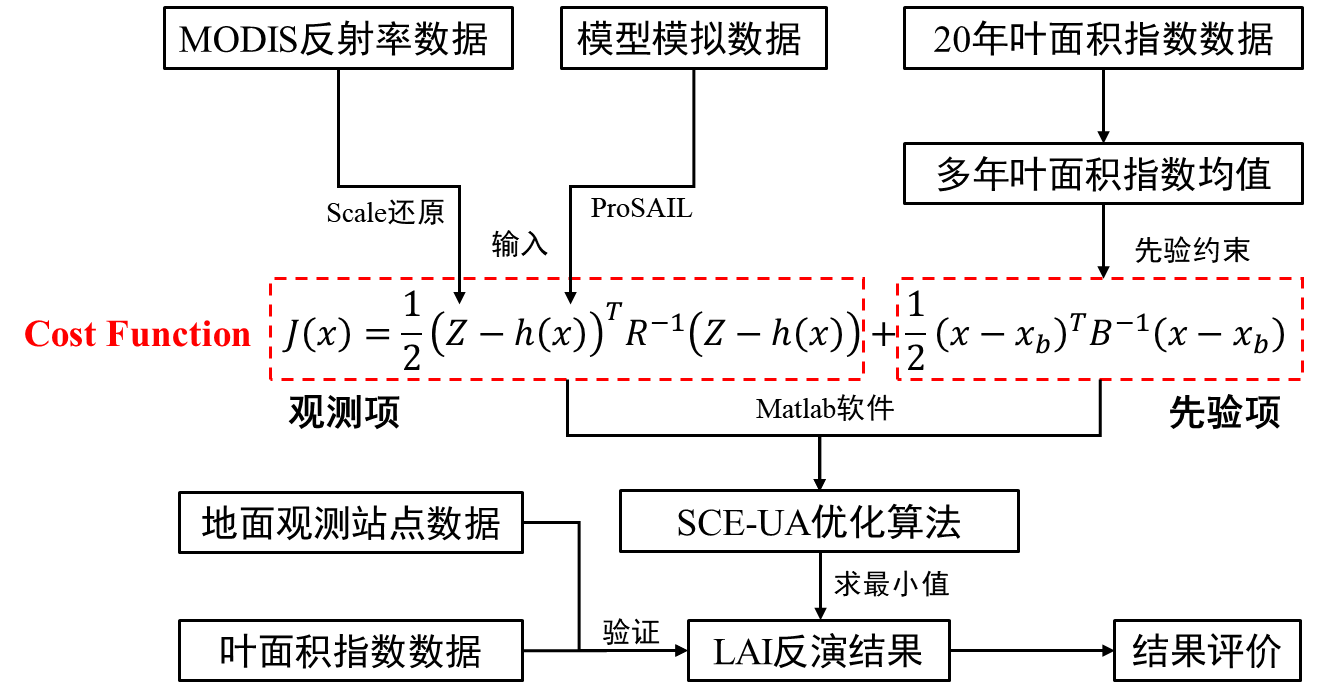
图 基于物理模型的LAI反演框架
站点所在像元一年的LAI反演的方式与上面类似,只是将空间上的逐像元反演转化为单个像元在时间序列上的反演。只需获取像元点的MODIS波段反射率数据即可。
(2)ProSAIL模型介绍
本次实习用到的模型为PROSAIL模型,综合课程讲解和文献资料,现对模型介绍如下:
随着光学遥感技术的发展,辐射传输模型致力于理解植物冠层对光的截获,并根据生物物理特征解释植被反射率。PROSAIL模型便是一种经典的辐射传输模型,由PROSPECT叶片光学特性模型和 SAILH 冠层结构模型耦合得到,目前已被广泛用于研究太阳辐射域内植物冠层的光谱和方向反射率,以及生物物理化学参数反演等研究。
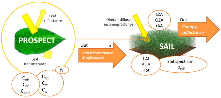
图 PROSAIL模型参数示意图
ProSAIL模型模拟的过程采用ProSAI_5B包进行,需要从其他渠道获取,如您有需要,也可以私信小编进行获取。
(3)SCE-UA算法介绍
SCE-UA算法由美国亚利桑那州大学水文与水资源系的Qingyun Duan博士提出。它的基本原理是通过把参数空间里的种群分成若干个子群,每个子群内部用单纯形的操作沿着下降方向搜索,从而在局部快速逼近更优解。SCE-UA综合了确定性搜索、随机搜索和生物竞争进化等方法的优点, 引入种群概念, 复合形点在可行域内随机生成和竞争演化[2-4]。
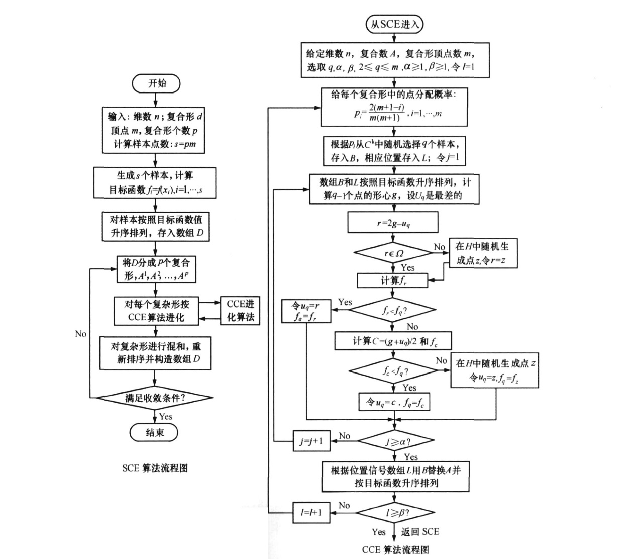
图 SCE-UA算法流程图(宋星原等,2009)
SCE-UA算法的实现过程主要通过老师分享的代码包来实现,通过调用编写的代价函数,执行迭代过程。站点小区域的主程序如下:
%% ========================================================================
% 草地LAI反演 - 标准贝叶斯公式 + SCE-UA算法 - 完整版
%
% 代价函数: J(x) = 1/2*(z-h(x))'*R^(-1)*(z-h(x)) + 1/2*(x-x_b)'*B^(-1)*(x-x_b)
% 优化算法: SCE-UA (Shuffled Complex Evolution)
% 站点: Wankama 2005草地
%% ========================================================================
clear; clc; close all;

fprintf('================================================================
');
fprintf('  草地LAI反演 - 标准贝叶斯公式 + SCE-UA算法
');
fprintf('================================================================
');
fprintf('站点: Wankama 2005
');
fprintf('日期: 2005-06-27
');
fprintf('================================================================
');

addpath('D:Duyan
emote_sensingLAIGrasslandGrassland_LAI_Inversion_PackageGrassland_LAI_Inversion_Package');

%% ========================================================================
% 1. 数据路径设置
%% ========================================================================
data_dir = 'D:Duyan
emote_sensingLAIGrasslandGEE_MODIS';
date_str = '20050627';

ref_files = cell(7,1);
for i = 1:7
    ref_files{i} = fullfile(data_dir, sprintf('MOD09A1_near_%s_ROI5km_b%d.tif', date_str, i));
end
modis_lai_file = fullfile(data_dir, sprintf('MOD15A2H_LAI_near_%s_ROI5km.tif', date_str));
prior_lai_file = fullfile(data_dir, 'MOD15A2H_LAI_priorMean_2002_2025_near_0627_ROI5km.tif');
ground_data_file = fullfile(data_dir, 'Wankama2005GroundData_latlon.xlsx');

output_dir = 'D:Duyan
emote_sensingLAIGrasslandGrassland_LAI_Inversion_PackageGrassland_LAI_Inversion_Packageoutputs';
if ~exist(output_dir, 'dir'), mkdir(output_dir); end

%% ========================================================================
% 2. 读取遥感数据
%% ========================================================================
fprintf('
正在读取数据...
');

[ref_b1, R] = readgeoraster(ref_files{1});
[nrows, ncols] = size(ref_b1);
fprintf('影像尺寸: %d x %d
', nrows, ncols);

reflectance = zeros(nrows, ncols, 7);
for i = 1:7
    reflectance(:,:,i) = readgeoraster(ref_files{i});
    fprintf('  波段%d读取完成
', i);
end

modis_lai = readgeoraster(modis_lai_file);
prior_lai_mean = readgeoraster(prior_lai_file);

% 处理无效值
reflectance(reflectance < 0 | reflectance > 1) = NaN;
modis_lai(modis_lai < 0 | modis_lai > 10) = NaN;
prior_lai_mean(prior_lai_mean < 0 | prior_lai_mean > 10) = NaN;

% 先验LAI统计
prior_valid = prior_lai_mean(~isnan(prior_lai_mean) & prior_lai_mean > 0);
fprintf('
先验LAI统计:
');
fprintf('  范围: [%.6f, %.6f]
', min(prior_valid), max(prior_valid));
fprintf('  均值: %.6f ± %.6f
', mean(prior_valid), std(prior_valid));

%% ========================================================================
% 3. 读取地面观测数据
%% ========================================================================
try
    ground_data = readtable(ground_data_file);
    fprintf('
地面观测样点: %d
', height(ground_data));
catch
    fprintf('
警告: 无法读取地面数据
');
    ground_data = [];
end

%% ========================================================================
% 4. 贝叶斯参数设置
%% ========================================================================
fprintf('
================================================================
');
fprintf('  贝叶斯反演参数设置
');
fprintf('================================================================
');

% PROSAIL模型参数 (草地)
fixed_params = struct();
fixed_params.N = 1.3;
fixed_params.Cab = 35;
fixed_params.Car = 9;
fixed_params.Cbrown = 0.0;
fixed_params.Cw = 0.010;
fixed_params.Cm = 0.004;
fixed_params.psoil = 0.4;
fixed_params.LIDFa = 70;
fixed_params.LIDFb = 0;
fixed_params.TypeLidf = 2;
fixed_params.hspot = 0.01;
fixed_params.tts = 30;
fixed_params.tto = 10;
fixed_params.psi = 0;

fprintf('
PROSAIL参数 (草地):
');
fprintf('  N=%.1f, Cab=%d, Cw=%.3f, LIDFa=%d°
', ...
        fixed_params.N, fixed_params.Cab, fixed_params.Cw, fixed_params.LIDFa);

% 协方差矩阵设置
obs_error_std = 0.03;
R_matrix = (obs_error_std^2) * eye(7);

prior_error_std = 0.5;
B_variance = prior_error_std^2;

fprintf('
协方差矩阵:
');
fprintf('  R: 观测误差协方差 (对角,标准差=%.3f)
', obs_error_std);
fprintf('  B: 背景误差方差 (%.4f)
', B_variance);

% LAI范围
lai_min = max(0.05, min(prior_valid) - 0.15);
lai_max = min(5.0, max(prior_valid) + 1.0);
fprintf('
LAI反演范围: [%.4f, %.4f]
', lai_min, lai_max);

% SCE-UA参数
sce_params = struct();
sce_params.maxn = 10000;
sce_params.kstop = 15;
sce_params.pcento = 0.01;
sce_params.peps = 0.001;
sce_params.ngs = 5;
sce_params.iseed = 123;
sce_params.iniflg = 1;

fprintf('
SCE-UA参数: maxn=%d, pcento=%.2f%%
', sce_params.maxn, sce_params.pcento);

%% ========================================================================
% 5. 逐像元LAI反演
%% ========================================================================
fprintf('
================================================================
');
fprintf('  开始逐像元LAI反演 (SCE-UA)
');
fprintf('================================================================
');

inverted_lai = nan(nrows, ncols);
convergence_flag = zeros(nrows, ncols);
cost_values = nan(nrows, ncols);

valid_pixels = 0;
total_pixels = nrows * ncols;

global CURRENT_OBS CURRENT_PRIOR FIXED_PARAMS_GLOBAL ...
       OBS_COV_MATRIX PRIOR_VARIANCE

FIXED_PARAMS_GLOBAL = fixed_params;
OBS_COV_MATRIX = R_matrix;
PRIOR_VARIANCE = B_variance;

tic;

for i = 1:nrows
    for j = 1:ncols
        if mod((i-1)*ncols + j, 20) == 0
            fprintf('  进度: %d/%d (%.1f%%)
', (i-1)*ncols+j, total_pixels, ...
                    ((i-1)*ncols+j)/total_pixels*100);
        end

        pixel_ref = squeeze(reflectance(i, j, :));

        if any(isnan(pixel_ref)) || all(pixel_ref == 0) || any(pixel_ref < 0.001)
            continue;
        end

        prior_lai_pixel = prior_lai_mean(i, j);
        if isnan(prior_lai_pixel) || prior_lai_pixel <= 0
            prior_lai_pixel = mean(prior_valid);
        end

        CURRENT_OBS = pixel_ref;
        CURRENT_PRIOR = prior_lai_pixel;
        lai_init = prior_lai_pixel;

        try
            [best_lai, best_cost, exitflag] = sceua(@functn, ...
                lai_init, lai_min, lai_max, ...
                sce_params.maxn, sce_params.kstop, ...
                sce_params.pcento, sce_params.peps, ...
                sce_params.ngs, sce_params.iseed, ...
                sce_params.iniflg);

            if isnan(best_lai) || isinf(best_cost) || best_cost > 1e10
                best_lai = prior_lai_pixel;
                exitflag = -1;
            end

            best_lai = max(lai_min, min(lai_max, best_lai));

            inverted_lai(i, j) = best_lai;
            cost_values(i, j) = best_cost;
            convergence_flag(i, j) = (exitflag >= 0);
            valid_pixels = valid_pixels + 1;

        catch
            inverted_lai(i, j) = prior_lai_pixel;
        end
    end
end

elapsed_time = toc;

fprintf('
反演完成! 用时: %.1f分钟
', elapsed_time/60);
fprintf('  有效像元: %d/%d (%.1f%%)
', valid_pixels, total_pixels, ...
        valid_pixels/total_pixels*100);

valid_lai = inverted_lai(~isnan(inverted_lai) & inverted_lai > 0);
fprintf('
反演LAI统计:
');
fprintf('  范围: [%.6f, %.6f]
', min(valid_lai), max(valid_lai));
fprintf('  均值: %.6f ± %.6f
', mean(valid_lai), std(valid_lai));

converged = sum(convergence_flag(:));
fprintf('
收敛率: %.1f%%
', converged/valid_pixels*100);

%% ========================================================================
% 6. 保存结果
%% ========================================================================
fprintf('
正在保存结果...
');

geotiffwrite(fullfile(output_dir, sprintf('Grassland_Bayesian_LAI_%s.tif', date_str)), ...
             inverted_lai, R);
geotiffwrite(fullfile(output_dir, sprintf('Grassland_Bayesian_Cost_%s.tif', date_str)), ...
             cost_values, R);
geotiffwrite(fullfile(output_dir, sprintf('Grassland_Bayesian_Convergence_%s.tif', date_str)), ...
             convergence_flag, R);

%% ========================================================================
% 7. 生成所需图表
%% ========================================================================
fprintf('
================================================================
');
fprintf('  生成可视化图表
');
fprintf('================================================================
');

% ------------------------------------------------------------------------
% 图1: 四张LAI对比图 (反演、MODIS、先验、差值)
% ------------------------------------------------------------------------
fprintf('  生成图1: LAI对比图...
');

figure('Position', [100, 100, 1800, 900]);

% 子图1: 反演LAI
subplot(2,2,1);
imagesc(inverted_lai);
h1 = colorbar;
ylabel(h1, 'LAI', 'FontSize', 10);
inv_min = min(valid_lai); inv_max = max(valid_lai);
caxis([inv_min*0.95 inv_max*1.05]);
title(sprintf('反演LAI (贝叶斯+SCE-UA)
范围: [%.4f, %.4f]', inv_min, inv_max), ...
      'FontSize', 12, 'FontWeight', 'bold');
axis image;
colormap(jet);
xlabel(sprintf('均值: %.4f, 标准差: %.4f', mean(valid_lai), std(valid_lai)), ...
       'FontSize', 10);

% 子图2: MODIS LAI
subplot(2,2,2);
imagesc(modis_lai);
h2 = colorbar;
ylabel(h2, 'LAI', 'FontSize', 10);
modis_valid = modis_lai(~isnan(modis_lai) & modis_lai > 0);
modis_min = min(modis_valid); modis_max = max(modis_valid);
caxis([modis_min*0.95 modis_max*1.05]);
title(sprintf('MODIS LAI产品
范围: [%.4f, %.4f]', modis_min, modis_max), ...
      'FontSize', 12, 'FontWeight', 'bold');
axis image;
colormap(jet);
xlabel(sprintf('均值: %.4f, 标准差: %.4f', mean(modis_valid), std(modis_valid)), ...
       'FontSize', 10);

% 子图3: 先验LAI (多年均值)
subplot(2,2,3);
imagesc(prior_lai_mean);
h3 = colorbar;
ylabel(h3, 'LAI', 'FontSize', 10);
prior_min = min(prior_valid); prior_max = max(prior_valid);
caxis([prior_min*0.95 prior_max*1.05]);
title(sprintf('先验LAI (多年均值 2002-2025)
范围: [%.6f, %.6f]', prior_min, prior_max), ...
      'FontSize', 12, 'FontWeight', 'bold');
axis image;
colormap(jet);
xlabel(sprintf('均值: %.6f, 标准差: %.6f', mean(prior_valid), std(prior_valid)), ...
       'FontSize', 10);

% 子图4: 差值图 (反演 - MODIS)
subplot(2,2,4);
diff_lai = inverted_lai - modis_lai;
imagesc(diff_lai);
h4 = colorbar;
ylabel(h4, 'LAI差值', 'FontSize', 10);
diff_valid = diff_lai(~isnan(diff_lai));
diff_abs_max = max(abs(diff_valid));
caxis([-diff_abs_max diff_abs_max]);
title(sprintf('差值图 (反演LAI - MODIS LAI)
范围: [%.4f, %.4f]', ...
      min(diff_valid), max(diff_valid)), ...
      'FontSize', 12, 'FontWeight', 'bold');
axis image;
colormap(gca, redblue);
xlabel(sprintf('均值: %.4f, 标准差: %.4f', mean(diff_valid), std(diff_valid)), ...
       'FontSize', 10);

sgtitle('草地LAI反演结果对比 (标准贝叶斯公式+SCE-UA)', ...
        'FontSize', 14, 'FontWeight', 'bold');

saveas(gcf, fullfile(output_dir, 'Grassland_Bayesian_LAI_Comparison.png'));
fprintf('    已保存: Grassland_Bayesian_LAI_Comparison.png
');

% ------------------------------------------------------------------------
% 图2: 反演LAI直方图
% ------------------------------------------------------------------------
fprintf('  生成图2: 反演LAI直方图...
');

figure('Position', [100, 100, 900, 700]);
histogram(valid_lai, 30, 'FaceColor', [0.2 0.6 0.8], 'EdgeColor', 'black');
hold on;

% 添加统计线
xline(mean(valid_lai), 'r--', 'LineWidth', 2, 'Label', sprintf('均值: %.4f', mean(valid_lai)));
xline(median(valid_lai), 'g--', 'LineWidth', 2, 'Label', sprintf('中位数: %.4f', median(valid_lai)));

xlabel('LAI', 'FontSize', 12, 'FontWeight', 'bold');
ylabel('频数', 'FontSize', 12, 'FontWeight', 'bold');
title('反演LAI分布直方图', 'FontSize', 14, 'FontWeight', 'bold');
grid on;

% 添加统计信息文本框
dim = [0.15 0.7 0.3 0.2];
str = {sprintf('样本数: %d', length(valid_lai)), ...
       sprintf('范围: [%.4f, %.4f]', min(valid_lai), max(valid_lai)), ...
       sprintf('均值: %.6f', mean(valid_lai)), ...
       sprintf('标准差: %.6f', std(valid_lai)), ...
       sprintf('中位数: %.6f', median(valid_lai)), ...
       sprintf('四分位距: %.6f', iqr(valid_lai))};
annotation('textbox', dim, 'String', str, 'FitBoxToText', 'on', ...
           'BackgroundColor', 'white', 'EdgeColor', 'black', 'FontSize', 10);

saveas(gcf, fullfile(output_dir, 'Grassland_Bayesian_LAI_Histogram.png'));
fprintf('    已保存: Grassland_Bayesian_LAI_Histogram.png
');

% ------------------------------------------------------------------------
% 图3: 散点图1 - 反演LAI vs MODIS LAI
% ------------------------------------------------------------------------
fprintf('  生成图3: 反演LAI vs MODIS LAI散点图...
');

valid_mask = ~isnan(inverted_lai) & ~isnan(modis_lai) & ...
             inverted_lai > 0 & modis_lai > 0;
inv_lai_vec = inverted_lai(valid_mask);
modis_lai_vec = modis_lai(valid_mask);

figure('Position', [100, 100, 900, 700]);
scatter(modis_lai_vec, inv_lai_vec, 35, 'filled', 'MarkerFaceAlpha', 0.6);
hold on;

% 自适应坐标轴
all_lai = [inv_lai_vec; modis_lai_vec];
axis_min = max(0, min(all_lai) * 0.90);
axis_max = max(all_lai) * 1.10;

% 1:1线
plot([axis_min axis_max], [axis_min axis_max], 'r--', 'LineWidth', 2.5);

% 线性拟合
p = polyfit(modis_lai_vec, inv_lai_vec, 1);
x_fit = linspace(axis_min, axis_max, 100);
y_fit = polyval(p, x_fit);
plot(x_fit, y_fit, 'b-', 'LineWidth', 2);

% 统计指标
rmse = sqrt(mean((inv_lai_vec - modis_lai_vec).^2));
bias = mean(inv_lai_vec - modis_lai_vec);
r = corrcoef(inv_lai_vec, modis_lai_vec);
r2 = r(1,2)^2;
mae = mean(abs(inv_lai_vec - modis_lai_vec));

xlabel('MODIS LAI', 'FontSize', 13, 'FontWeight', 'bold');
ylabel('反演LAI (贝叶斯+SCE-UA)', 'FontSize', 13, 'FontWeight', 'bold');
title('反演LAI vs MODIS LAI', 'FontSize', 14, 'FontWeight', 'bold');
grid on;
axis equal;
xlim([axis_min axis_max]);
ylim([axis_min axis_max]);

% 统计信息
text_x = axis_min + (axis_max - axis_min) * 0.05;
text_y = axis_max - (axis_max - axis_min) * 0.30;
text_str = sprintf(['R² = %.4f
' ...
                    'RMSE = %.6f
' ...
                    'MAE = %.6f
' ...
                    'Bias = %.6f
' ...
                    'y = %.3fx + %.3f
' ...
                    'N = %d'], ...
                   r2, rmse, mae, bias, p(1), p(2), length(inv_lai_vec));
text(text_x, text_y, text_str, 'FontSize', 11, ...
     'BackgroundColor', 'white', 'EdgeColor', 'black', ...
     'VerticalAlignment', 'top');

legend('数据点', '1:1线', '拟合线', 'Location', 'southeast', 'FontSize', 10);

saveas(gcf, fullfile(output_dir, 'Grassland_Bayesian_Scatter_MODIS.png'));
fprintf('    已保存: Grassland_Bayesian_Scatter_MODIS.png
');

% ------------------------------------------------------------------------
% 图4: 散点图2 - 反演LAI vs 地面观测LAI
% ------------------------------------------------------------------------
if ~isempty(ground_data)
    fprintf('  生成图4: 反演LAI vs 地面观测LAI散点图...
');

    % 确定LAI列
    if ismember('LAItrue', ground_data.Properties.VariableNames)
        ground_lai_col = 'LAItrue';
    else
        lai_cols = ground_data.Properties.VariableNames(...
            contains(ground_data.Properties.VariableNames, 'LAI'));
        if ~isempty(lai_cols)
            ground_lai_col = lai_cols{1};
        else
            fprintf('    警告: 未找到地面LAI列
');
            ground_lai_col = '';
        end
    end

    if ~isempty(ground_lai_col)
        n_samples = height(ground_data);
        ground_lai = ground_data.(ground_lai_col);
        inv_lai_at_samples = zeros(n_samples, 1);

        for k = 1:n_samples
            lon = ground_data.Longitude(k);
            lat = ground_data.Latitude(k);
            [row, col] = geographicToDiscrete(R, lat, lon);

            if row >= 1 && row <= nrows && col >= 1 && col <= ncols
                inv_lai_at_samples(k) = inverted_lai(round(row), round(col));
            else
                inv_lai_at_samples(k) = NaN;
            end
        end

        valid_samples = ~isnan(inv_lai_at_samples) & ~isnan(ground_lai) & ...
                        inv_lai_at_samples > 0 & ground_lai > 0;
        inv_lai_samples = inv_lai_at_samples(valid_samples);
        ground_lai_valid = ground_lai(valid_samples);

        if sum(valid_samples) > 3
            figure('Position', [100, 100, 900, 700]);
            scatter(ground_lai_valid, inv_lai_samples, 100, 'filled', ...
                    'MarkerFaceAlpha', 0.7, 'MarkerEdgeColor', 'black');
            hold on;

            % 自适应坐标轴
            all_lai_g = [inv_lai_samples; ground_lai_valid];
            g_axis_min = max(0, min(all_lai_g) * 0.85);
            g_axis_max = max(all_lai_g) * 1.15;

            % 1:1线
            plot([g_axis_min g_axis_max], [g_axis_min g_axis_max], ...
                 'r--', 'LineWidth', 2.5);

            % 线性拟合
            p_g = polyfit(ground_lai_valid, inv_lai_samples, 1);
            x_fit_g = linspace(g_axis_min, g_axis_max, 100);
            y_fit_g = polyval(p_g, x_fit_g);
            plot(x_fit_g, y_fit_g, 'b-', 'LineWidth', 2);

            % 统计指标
            rmse_g = sqrt(mean((inv_lai_samples - ground_lai_valid).^2));
            bias_g = mean(inv_lai_samples - ground_lai_valid);
            r_g = corrcoef(inv_lai_samples, ground_lai_valid);
            r2_g = r_g(1,2)^2;
            mae_g = mean(abs(inv_lai_samples - ground_lai_valid));

            xlabel('地面观测LAI', 'FontSize', 13, 'FontWeight', 'bold');
            ylabel('反演LAI (贝叶斯+SCE-UA)', 'FontSize', 13, 'FontWeight', 'bold');
            title('反演LAI vs 地面观测LAI', 'FontSize', 14, 'FontWeight', 'bold');
            grid on;
            axis equal;
            xlim([g_axis_min g_axis_max]);
            ylim([g_axis_min g_axis_max]);

            % 统计信息
            text_x_g = g_axis_min + (g_axis_max - g_axis_min) * 0.05;
            text_y_g = g_axis_max - (g_axis_max - g_axis_min) * 0.35;
            text_str_g = sprintf(['R² = %.4f
' ...
                                  'RMSE = %.6f
' ...
                                  'MAE = %.6f
' ...
                                  'Bias = %.6f
' ...
                                  'y = %.3fx + %.3f
' ...
                                  'N = %d'], ...
                                 r2_g, rmse_g, mae_g, bias_g, p_g(1), p_g(2), sum(valid_samples));
            text(text_x_g, text_y_g, text_str_g, 'FontSize', 11, ...
                 'BackgroundColor', 'white', 'EdgeColor', 'black', ...
                 'VerticalAlignment', 'top');

            legend('数据点', '1:1线', '拟合线', 'Location', 'southeast', 'FontSize', 10);

            saveas(gcf, fullfile(output_dir, 'Grassland_Bayesian_Scatter_Ground.png'));
            fprintf('    已保存: Grassland_Bayesian_Scatter_Ground.png
');

            fprintf('
与地面观测对比:
');
            fprintf('  RMSE: %.6f
', rmse_g);
            fprintf('  MAE:  %.6f
', mae_g);
            fprintf('  Bias: %.6f
', bias_g);
            fprintf('  R²:   %.6f
', r2_g);
        end
    end
else
    fprintf('  跳过图4: 无地面观测数据
');
end

%% ========================================================================
% 8. 保存统计报告
%% ========================================================================
fprintf('
保存统计报告...
');

results_table = table();
results_table.Metric = {'Obs_Error_Std'; 'Prior_Error_Std'; ...
                        'RMSE_MODIS'; 'MAE_MODIS'; 'Bias_MODIS'; 'R2_MODIS'; ...
                        'Inv_LAI_Min'; 'Inv_LAI_Max'; 'Inv_LAI_Mean'; 'Inv_LAI_Std'; ...
                        'Prior_LAI_Min'; 'Prior_LAI_Max'; 'Prior_LAI_Mean'; 'Prior_LAI_Std'; ...
                        'Valid_Pixels'; 'Convergence_Rate'; 'Elapsed_Time_Min'};
results_table.Value = [obs_error_std; prior_error_std; ...
                       rmse; mae; bias; r2; ...
                       min(valid_lai); max(valid_lai); mean(valid_lai); std(valid_lai); ...
                       min(prior_valid); max(prior_valid); mean(prior_valid); std(prior_valid); ...
                       valid_pixels; converged/valid_pixels; elapsed_time/60];

writetable(results_table, fullfile(output_dir, 'Grassland_Bayesian_Statistics.csv'));

fprintf('
================================================================
');
fprintf('  程序运行完成!
');
fprintf('================================================================
');
fprintf('算法: 标准贝叶斯公式 + SCE-UA
');
fprintf('反演LAI: [%.6f, %.6f], 均值=%.6f
', ...
        min(valid_lai), max(valid_lai), mean(valid_lai));
fprintf('与MODIS对比: RMSE=%.6f, R²=%.6f
', rmse, r2);
fprintf('收敛率: %.1f%%
', converged/valid_pixels*100);
fprintf('用时: %.1f分钟
', elapsed_time/60);
fprintf('================================================================
');
fprintf('
生成的图表:
');
fprintf('  1. Grassland_Bayesian_LAI_Comparison.png  (4图对比)
');
fprintf('  2. Grassland_Bayesian_LAI_Histogram.png   (直方图)
');
fprintf('  3. Grassland_Bayesian_Scatter_MODIS.png   (vs MODIS)
');
fprintf('  4. Grassland_Bayesian_Scatter_Ground.png  (vs 地面)
');
fprintf('================================================================
');

% 辅助函数: 红蓝色图
function map = redblue(m)
    if nargin < 1
        m = size(get(gcf,'colormap'),1);
    end
    r = (0:m-1)'/max(m-1,1);
    map = [max(0,1-2*r) ones(m,1)-2*abs(r-0.5) max(0,2*r-1)];
end
如果你需要反演某个像元一年的LAI的时间序列,可以使用如下的代码进行,二者还是比较类似的
%% ========================================================================
% LAI时间序列反演 - 单像元全年反演
%% ========================================================================
% 功能: 基于PROSAIL模型和SCE-UA优化算法反演单像元全年LAI时间序列
% 输入: MOD09A1反射率CSV + MOD15A2H LAI CSV
% 输出: 反演LAI时间序列 + 对比图表 + 精度统计
%
% 作者: Claude
% 日期: 2026-01-31
%% ========================================================================

clear; clc; close all;
fprintf('========================================
');
fprintf('LAI时间序列反演程序
');
fprintf('========================================
');

%% ========================================================================
% 1. 设置数据路径
%% ========================================================================
% 修改这里为你的数据路径
data_dir = 'D:Duyan
emote_sensingLAIForest';

% 输入文件
refl_file = fullfile(data_dir, 'MOD09A1_Point_2020_b1_b7_scaled.csv');
lai_file = fullfile(data_dir, 'MOD15A2H_LAI_Point_2020.csv');

% 输出目录
output_dir = fullfile(data_dir, 'output_timeseries');
if ~exist(output_dir, 'dir')
    mkdir(output_dir);
end

fprintf('数据目录: %s
', data_dir);
fprintf('输出目录: %s
', output_dir);

%% ========================================================================
% 2. 读取时间序列数据
%% ========================================================================
fprintf('
========================================
');
fprintf('读取时间序列数据
');
fprintf('========================================
');

% 读取反射率数据
fprintf('读取MOD09A1反射率数据...
');
refl_data = readtable(refl_file);
fprintf('  时间点数: %d
', height(refl_data));

% 读取MODIS LAI数据
fprintf('读取MOD15A2H LAI数据...
');
lai_data = readtable(lai_file);
fprintf('  时间点数: %d
', height(lai_data));

% 检查时间点数量是否一致
if height(refl_data) ~= height(lai_data)
    warning('反射率和LAI数据时间点数量不一致!');
end

% 提取时间序列
n_times = height(refl_data);
dates = refl_data.system_index;  % 时间列

% 提取7个波段反射率
b1 = refl_data.b1;
b2 = refl_data.b2;
b3 = refl_data.b3;
b4 = refl_data.b4;
b5 = refl_data.b5;
b6 = refl_data.b6;
b7 = refl_data.b7;

% 提取MODIS LAI
modis_lai = lai_data.LAI;

fprintf('数据读取完成!
');
fprintf('  时间范围: %s 至 %s
', string(dates(1)), string(dates(end)));
fprintf('  MODIS LAI范围: %.2f - %.2f
', min(modis_lai), max(modis_lai));

%% ========================================================================
% 3. 设置PROSAIL模型固定参数
%% ========================================================================
fprintf('
========================================
');
fprintf('设置PROSAIL模型参数
');
fprintf('========================================
');

% 叶片参数 (根据森林类型调整)
fixed_params.N = 1.5;           % 叶片结构参数
fixed_params.Cab = 45;          % 叶绿素含量 (μg/cm²) [30-60]
fixed_params.Car = 8;           % 类胡萝卜素含量 (μg/cm²)
fixed_params.Cw = 0.015;        % 等效水厚度 (cm) [0.01-0.03]
fixed_params.Cm = 0.005;        % 干物质含量 (g/cm²)
fixed_params.Cbrown = 0;        % 褐色素含量

% 冠层结构参数
fixed_params.LIDFa = 57;        % 平均叶倾角 (度) [40-70]
fixed_params.TypeLidf = 2;      % 叶倾角分布类型 (2=椭球分布)
fixed_params.lai = 3.0;         % LAI初值 (将被优化)

% 土壤和背景
fixed_params.psoil = 1.0;       % 土壤亮度系数

% 观测几何 (根据实际情况调整)
fixed_params.tts = 30;          % 太阳天顶角 (度)
fixed_params.tto = 10;          % 观测天顶角 (度)
fixed_params.psi = 0;           % 相对方位角 (度)

fprintf('PROSAIL参数设置完成
');
fprintf('  叶绿素: %.1f μg/cm²
', fixed_params.Cab);
fprintf('  水分: %.4f cm
', fixed_params.Cw);
fprintf('  平均叶倾角: %.1f°
', fixed_params.LIDFa);

%% ========================================================================
% 4. 设置SCE-UA优化参数
%% ========================================================================
fprintf('
========================================
');
fprintf('设置优化算法参数
');
fprintf('========================================
');

% SCE-UA参数
sce_params.maxn = 5000;         % 最大迭代次数 [3000-8000]
sce_params.kstop = 10;          % 收敛判断次数
sce_params.pcento = 0.1;        % 收敛阈值 (百分比)
sce_params.peps = 0.001;        % 参数空间收敛阈值
sce_params.ngs = 5;             % 复形数量 [3-7]
sce_params.iseed = 0;           % 随机种子
sce_params.iniflg = 1;          % 初始化标志

% LAI参数范围
lai_min = 0.1;                  % LAI最小值
lai_max = 7.0;                  % LAI最大值

fprintf('优化参数设置完成
');
fprintf('  最大迭代: %d
', sce_params.maxn);
fprintf('  LAI范围: [%.1f, %.1f]
', lai_min, lai_max);

%% ========================================================================
% 5. 定义全局变量供代价函数使用
%% ========================================================================
global obs_refl fixed_prosail_params

%% ========================================================================
% 6. 时间序列反演循环
%% ========================================================================
fprintf('
========================================
');
fprintf('开始时间序列反演
');
fprintf('========================================
');

% 初始化结果数组
inverted_lai = zeros(n_times, 1);
convergence_flag = zeros(n_times, 1);
iteration_count = zeros(n_times, 1);

% 记录开始时间
tic;

% 逐时间点反演
for t = 1:n_times
    if mod(t, 5) == 0 || t == 1
        fprintf('
处理时间点 %d/%d (%.1f%%)...
', t, n_times, 100*t/n_times);
    end

    % 提取当前时间点的7波段反射率
    current_refl = [b1(t); b2(t); b3(t); b4(t); b5(t); b6(t); b7(t)];

    % 检查数据有效性
    if any(isnan(current_refl)) || any(current_refl < 0) || any(current_refl > 1)
        fprintf('  警告: 时间点%d数据无效,跳过
', t);
        inverted_lai(t) = NaN;
        convergence_flag(t) = -1;
        continue;
    end

    % 设置全局变量
    obs_refl = current_refl;
    fixed_prosail_params = fixed_params;

    % 初始LAI值
    if t == 1
        % 第一个时间点:使用MODIS LAI作为初值
        x0 = modis_lai(t);
    else
        % 后续时间点:使用前一个反演结果作为初值
        if ~isnan(inverted_lai(t-1)) && inverted_lai(t-1) > 0
            x0 = inverted_lai(t-1);
        else
            x0 = modis_lai(t);
        end
    end

    % 确保初值在范围内
    x0 = max(lai_min, min(lai_max, x0));

    % 调用SCE-UA优化算法
    bl = lai_min;  % 下界
    bu = lai_max;  % 上界

    [bestx, bestf, icall, ~] = sceua(x0, bl, bu, sce_params.maxn, ...
        sce_params.kstop, sce_params.pcento, sce_params.peps, ...
        sce_params.ngs, sce_params.iseed, sce_params.iniflg);

    % 保存结果
    inverted_lai(t) = bestx;
    iteration_count(t) = icall;

    % 判断收敛
    if bestf < 0.01  % 代价函数很小,认为收敛
        convergence_flag(t) = 1;
    else
        convergence_flag(t) = 0;
        fprintf('  警告: 时间点%d未完全收敛 (代价函数=%.4f)
', t, bestf);
    end

    if mod(t, 5) == 0 || t == 1
        fprintf('  反演LAI: %.3f, MODIS LAI: %.3f, 迭代次数: %d
', ...
            inverted_lai(t), modis_lai(t), icall);
    end
end

% 记录结束时间
elapsed_time = toc;

fprintf('
========================================
');
fprintf('反演完成!
');
fprintf('========================================
');
fprintf('总耗时: %.1f 秒 (平均 %.2f 秒/点)
', elapsed_time, elapsed_time/n_times);
fprintf('收敛点数: %d/%d (%.1f%%)
', sum(convergence_flag==1), n_times, ...
    100*sum(convergence_flag==1)/n_times);
fprintf('平均迭代次数: %.0f
', mean(iteration_count(convergence_flag==1)));

%% ========================================================================
% 7. 保存结果到CSV
%% ========================================================================
fprintf('
========================================
');
fprintf('保存反演结果
');
fprintf('========================================
');

% 创建结果表格
results_table = table(dates, modis_lai, inverted_lai, convergence_flag, ...
    'VariableNames', {'Date', 'MODIS_LAI', 'Inverted_LAI', 'Converged'});

% 保存为CSV
output_csv = fullfile(output_dir, 'LAI_TimeSeries_Results_2020.csv');
writetable(results_table, output_csv);
fprintf('结果已保存: %s
', output_csv);

%% ========================================================================
% 8. 精度验证
%% ========================================================================
fprintf('
========================================
');
fprintf('精度验证统计
');
fprintf('========================================
');

% 仅使用收敛的点进行统计
valid_idx = (convergence_flag == 1) & ~isnan(inverted_lai) & ~isnan(modis_lai);
inv_valid = inverted_lai(valid_idx);
modis_valid = modis_lai(valid_idx);

if sum(valid_idx) < 3
    warning('有效数据点太少,无法进行统计分析!');
else
    % 计算精度指标
    rmse = sqrt(mean((inv_valid - modis_valid).^2));
    bias = mean(inv_valid - modis_valid);
    mae = mean(abs(inv_valid - modis_valid));

    % 计算R²
    ss_res = sum((inv_valid - modis_valid).^2);
    ss_tot = sum((modis_valid - mean(modis_valid)).^2);
    r2 = 1 - ss_res/ss_tot;

    % 显示统计结果
    fprintf('有效样本数: %d
', sum(valid_idx));
    fprintf('RMSE: %.4f
', rmse);
    fprintf('Bias: %.4f
', bias);
    fprintf('MAE: %.4f
', mae);
    fprintf('R²: %.4f
', r2);

    % 保存统计结果
    stats_table = table({'RMSE'; 'Bias'; 'MAE'; 'R²'; 'Valid_Points'}, ...
        [rmse; bias; mae; r2; sum(valid_idx)], ...
        'VariableNames', {'Metric', 'Value'});

    stats_csv = fullfile(output_dir, 'Validation_Statistics.csv');
    writetable(stats_table, stats_csv);
    fprintf('统计结果已保存: %s
', stats_csv);
end

%% ========================================================================
% 9. 绘制时间序列对比图
%% ========================================================================
fprintf('
========================================
');
fprintf('生成可视化图表
');
fprintf('========================================
');

% 转换日期格式(如果可能)
try
    date_nums = datenum(dates);
catch
    date_nums = 1:n_times;  % 如果日期转换失败,使用序号
end

% 图1: 时间序列对比图
figure('Position', [100, 100, 1200, 500]);
plot(date_nums, modis_lai, 'b-o', 'LineWidth', 1.5, 'MarkerSize', 6, ...
    'DisplayName', 'MODIS LAI');
hold on;
plot(date_nums, inverted_lai, 'r-s', 'LineWidth', 1.5, 'MarkerSize', 6, ...
    'DisplayName', 'Inverted LAI');

% 标记未收敛的点
unconverged_idx = (convergence_flag ~= 1);
if any(unconverged_idx)
    plot(date_nums(unconverged_idx), inverted_lai(unconverged_idx), ...
        'kx', 'MarkerSize', 10, 'LineWidth', 2, 'DisplayName', 'Not Converged');
end

hold off;
xlabel('Date', 'FontSize', 12, 'FontWeight', 'bold');
ylabel('LAI', 'FontSize', 12, 'FontWeight', 'bold');
title('LAI Time Series Comparison - 2020', 'FontSize', 14, 'FontWeight', 'bold');
legend('Location', 'best', 'FontSize', 11);
grid on;

% 设置日期刻度(如果日期转换成功)
if exist('datenum', 'builtin')
    datetick('x', 'mmm-yy', 'keepticks');
end

saveas(gcf, fullfile(output_dir, 'LAI_TimeSeries_Comparison.png'));
fprintf('  时间序列图已保存
');

%% ========================================================================
% 10. 绘制散点图
%% ========================================================================
if sum(valid_idx) >= 3
    figure('Position', [100, 100, 600, 600]);
    scatter(modis_valid, inv_valid, 80, 'b', 'filled', 'MarkerEdgeColor', 'k');
    hold on;

    % 1:1线
    min_val = min([modis_valid; inv_valid]);
    max_val = max([modis_valid; inv_valid]);
    plot([min_val, max_val], [min_val, max_val], 'k--', 'LineWidth', 1.5);

    % 线性拟合
    p = polyfit(modis_valid, inv_valid, 1);
    fit_x = linspace(min_val, max_val, 100);
    fit_y = polyval(p, fit_x);
    plot(fit_x, fit_y, 'r-', 'LineWidth', 2);

    hold off;
    xlabel('MODIS LAI', 'FontSize', 12, 'FontWeight', 'bold');
    ylabel('Inverted LAI', 'FontSize', 12, 'FontWeight', 'bold');
    title('LAI Validation Scatter Plot', 'FontSize', 14, 'FontWeight', 'bold');
    grid on;
    axis equal;
    xlim([min_val, max_val]);
    ylim([min_val, max_val]);

    % 添加统计信息
    text_str = sprintf('R² = %.4f
RMSE = %.4f
Bias = %.4f
N = %d', ...
        r2, rmse, bias, sum(valid_idx));
    text(0.05, 0.95, text_str, 'Units', 'normalized', 'FontSize', 11, ...
        'BackgroundColor', 'white', 'VerticalAlignment', 'top');

    saveas(gcf, fullfile(output_dir, 'LAI_Scatter_Plot.png'));
    fprintf('  散点图已保存
');
end

%% ========================================================================
% 11. 绘制残差分析图
%% ========================================================================
if sum(valid_idx) >= 3
    figure('Position', [100, 100, 1200, 400]);

    % 残差
    residuals = inv_valid - modis_valid;

    subplot(1, 2, 1);
    plot(date_nums(valid_idx), residuals, 'b-o', 'LineWidth', 1.5, 'MarkerSize', 6);
    hold on;
    yline(0, 'k--', 'LineWidth', 1.5);
    yline(mean(residuals), 'r--', 'LineWidth', 1.5, 'DisplayName', ...
        sprintf('Mean Bias = %.3f', bias));
    hold off;
    xlabel('Date', 'FontSize', 12, 'FontWeight', 'bold');
    ylabel('Residual (Inverted - MODIS)', 'FontSize', 12, 'FontWeight', 'bold');
    title('Residual Analysis', 'FontSize', 14, 'FontWeight', 'bold');
    legend('Location', 'best');
    grid on;
    if exist('datenum', 'builtin')
        datetick('x', 'mmm-yy', 'keepticks');
    end

    subplot(1, 2, 2);
    histogram(residuals, 15, 'FaceColor', 'b', 'EdgeColor', 'k');
    xlabel('Residual (Inverted - MODIS)', 'FontSize', 12, 'FontWeight', 'bold');
    ylabel('Frequency', 'FontSize', 12, 'FontWeight', 'bold');
    title('Residual Distribution', 'FontSize', 14, 'FontWeight', 'bold');
    grid on;

    saveas(gcf, fullfile(output_dir, 'LAI_Residual_Analysis.png'));
    fprintf('  残差分析图已保存
');
end

%% ========================================================================
% 完成
%% ========================================================================
fprintf('
========================================
');
fprintf('程序运行完成!
');
fprintf('========================================
');
fprintf('输出文件位于: %s
', output_dir);
fprintf('  1. LAI_TimeSeries_Results_2020.csv    - 反演结果CSV
');
fprintf('  2. Validation_Statistics.csv           - 精度统计
');
fprintf('  3. LAI_TimeSeries_Comparison.png       - 时间序列对比图
');
fprintf('  4. LAI_Scatter_Plot.png                - 散点验证图
');
fprintf('  5. LAI_Residual_Analysis.png           - 残差分析图
');
fprintf('========================================
');
上述代码的实现依赖于一些核心的代码包,可以私信小编联系。
5 反演结果
(1)站点附近小区域的LAI反演
本次选用以站点经纬度为中心点附近5km×5km的区域,通过全局优化算法展开函数求解,进行LAI反演,并将得到的结果和地面测量数据以及MODIS的反射率产品进行对比。得到的结果如下:
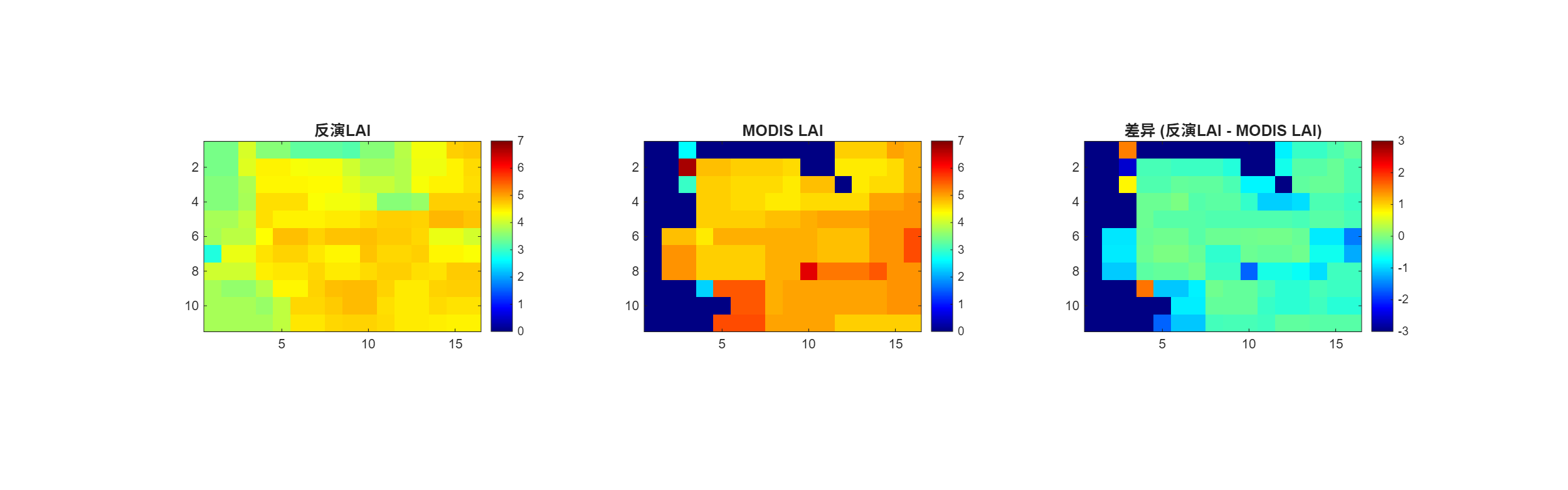
图 考虑先验信息下的反演结果-森林站点
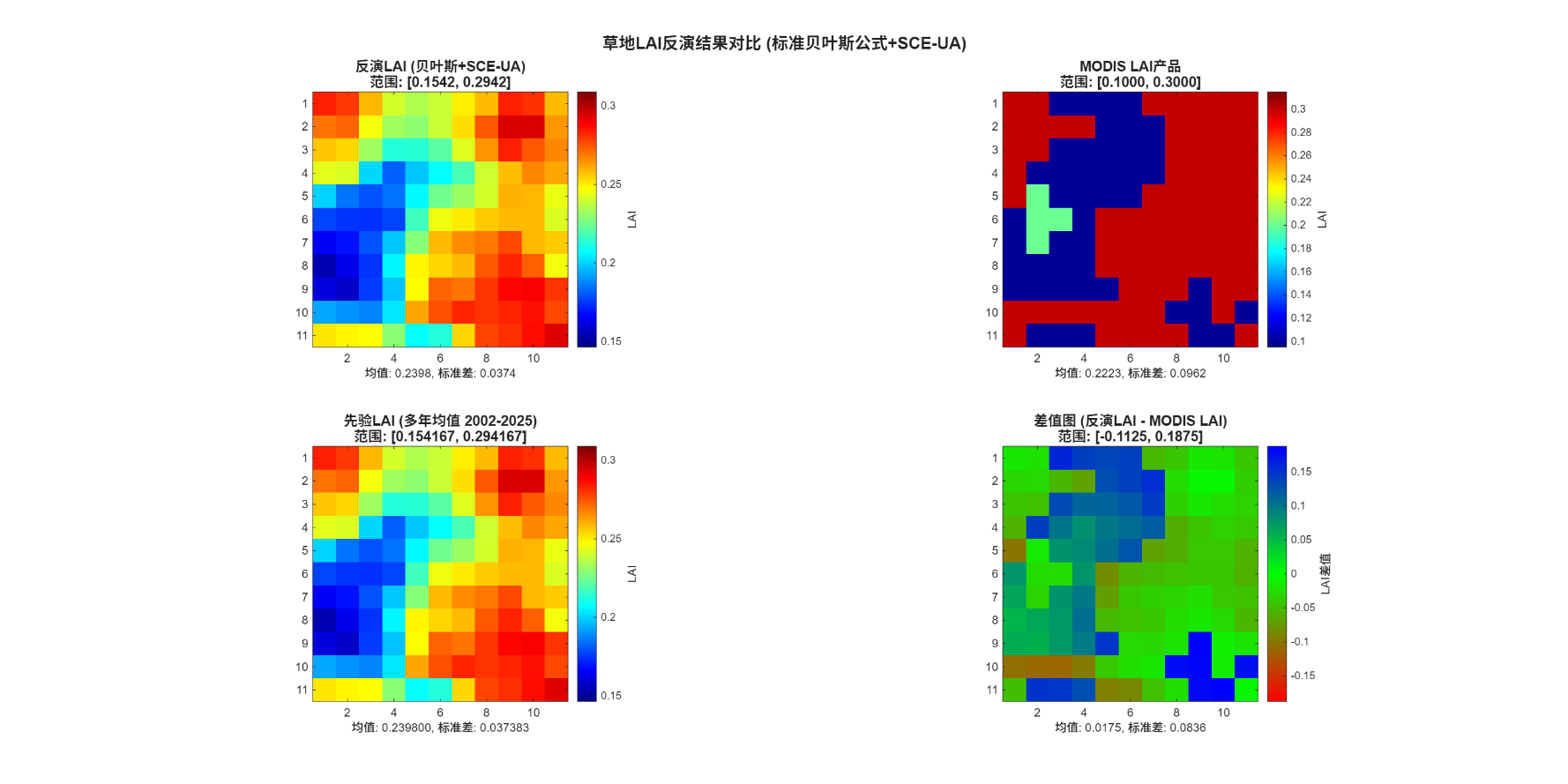
图 考虑先验信息下的反演结果-草地站点
(2)站点所在像元一年的LAI值反演
反演站点所在像元一年的时间序列时,实习过程用的代价函数并没有考虑先验信息。
从趋势上看,反演的LAI时间序列在趋势上基本吻合了MODIS产品的LAI时间序列。据图,发现夏季的反演效果相对较好,两条线比较接近,反演的LAI略低于MODIS的叶面积指数。同时两数据的差值最小,尤其是在7月-9月;冬季反演的的效果比较差,反演的LAI显著高于MODIS的产品。
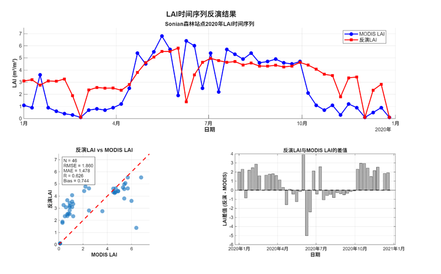
从指标评估来看,反演的LAI和MODIS提供的LAI拟合系数能够达到0.626,均方根误差为1.86,MAE为1.478,总体而言反演的精度相较于站点的小区域LAI精度要高。当然,如果能够纳入多年同一像元的LAI数据作为先验信息输入,或许能够进一步提供LAI模拟的精度。
6 学习总结
遥感反演是一项复杂的任务,病态反演问题告诉我们,实现完美的反演过程只是一种理想,我们工作的重心更应在于如何管理与约束算法求解过程的不确定性,尽管结果有待提高,但仍然是一次不错的尝试!
以上是本期关于遥感反演LAI指数的全部内容啦,欢迎交流!